
R Notebooks
An R Notebook is an R Markdown document with a special execution mode for interactive data analysis. Any R Markdown document can be used as a notebook, and R Notebooks can be rendered into the same publication-quality document formats as regular R Markdown files. By default, RStudio enables notebook mode on all R Markdown documents, so you can interact with any R Markdown document as though it were a notebook. R Notebooks, however, offer additional features that are not available in regular R Markdown documents.
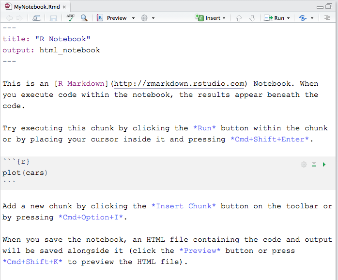
In RStudio, create a new R Notebook by clicking the File menu, then New File, and then select R Notebook. For this example we will save the notebook and give it a file name of MyNotebook.Rmd. Your editor pane should now look something like this:
(Click to enlarge.)
This is the R Studio template for an R Notebook. Kind of looks like regular R Markdown, doesn’t it? That’s because an R Notebook is an R Markdown document with code chunks that can be executed independently and interactively. Text and graphical output will appear immediately beneath the code chunk that produced it, in the editor window.
You can execute your notebook code chunks interactively by using the controls that appear in each chunk:
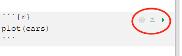
The rightmost arrow will run the current chunk. To the left of the run arrow is a down-pointing arrow that will run all of the chunks above the current chunk. The gear icon allows you to modify options for how each code chunk behaves. These same controls are also available in regular R Markdown documents.
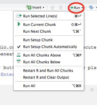
More options for running code chunks can be found in the Run menu on the editor toolbar:
A feature unique to R Notebooks is notebook Preview:
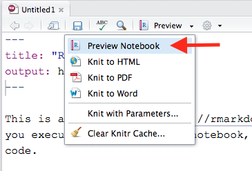
While an R notebook preview looks similar to a rendered R Markdown document, the notebook preview does not automatically execute and knit all of your code chunks, which is what happens when you render an R Markdown document. A notebook preview simply shows you a rendered copy of the Markdown text in your R Notebook along with the most recent chunk output. This allows you to efficiently develop R code in an R Notebook by iterating back and forth between coding and output until the code chunk is completed, without having to render the entire document each time you want to look at the output of a single code chunk.
Try previewing the R Notebook template before running the embedded code chunk. You’ll see just the text of the notebook in the Viewer pane. Then run the code chunk by clicking the Run arrow. A plot of the cars dataset (which comes with R) will appear immediately below the code chunk, not in the View pane, but right in the editor window. In the upper right corner of the plot window are tools for clearing the output, expanding or collapsing it (without clearing it), and for opening the graphic in an external window. If you leave the plot displayed, and then preview the notebook, you will now see the graphic included with the rendered text.
The YAML header in our R Notebook looks like this:
---
title: "R Notebook"
output: html_notebook
---
The output: html_notebook statement in the YAML header is what turns a regular R Markdown document into an R Notebook. So if you start out with an R Markdown document and then decide that you want to “upgrade” it to a notebook, just add output: html_notebook to the YAML header. This will turn your R Markdown document into an R Notebook and will also turn the Knit button into a Preview button. You will still have the option to knit the notebook completely into publication-quality output with all R text and graphical output. Just pull down the Preview button and you will see the knit options for HTML, PDF, and Word output.
Now that you have previewed MyNotebook.Rmd with the chunk output displayed, note that there is a file named MyNotebook.nb.html in your working directory. As discussed here, when a notebook .Rmd file is saved, the output: html_notebook statement in the YAML header causes an .nb.html having the same name as the notebook to be saved as well (the nb stands for notebook). This file is a self-contained HTML document having both a rendered copy of the notebook with all current chunk outputs (suitable for display on a website) plus a copy of the notebook .Rmd source file itself.
Open your RStudio Files pane, and click on MyNotebook.nb.html in the list of files. Choose to view the file in a web browser. It should look something like this:
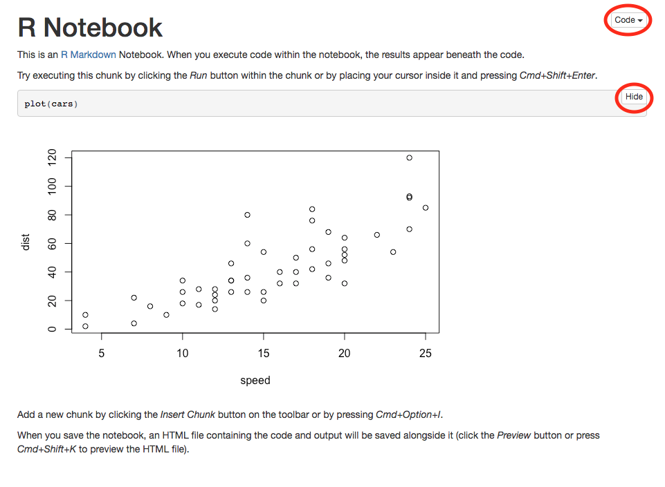
(Click to enlarge.)
In this web page, there is a button labeled Hide that you can use to show and hide the code that produced the plot. There is also a button labeled Code that lets you show and hide all of the code and also lets you download the original notebook .Rmd file.
The nb.html files are an excellent way to archive and share R notebooks. Anyone with access to an nb.html file has a complete package of the rendered text of the notebook, all of the tabular and graphical output from the code chunks, and a copy of the original R Notebook .Rmd file. Because the nb.html file can be viewed in any web browser, a person does not have to have R or RStudio in order to view the notebook, the code, or the output. However, if one of your collaborators does have RStudio, they can open the nb.html file directly using the File|Open File... dialog of RStudio to resume work on the notebook with all output intact. This will extract the .Rmd file into a new RStudio editor tab, extract the chunk outputs from the .nb.html file, and place them appropriately in the editor.
Only R Notebooks (which have at least one of the output formats in the YAML header listed as html_notebook) can produce a companion .nb.html file. Regular, non-notebook R Markdown files can have inline chunk output (the chunk output appears immediately below the chunk, in the editor) but they do not produce an .nb.html file.