RStudio as a Research and Writing Platform

Rendering Documents in RStudio

We will first examine RStudio as a platform for writing plain text R Markdown documents, inserting bibliographic citations, producing formatted bibliographies, and rendering the Markdown document into publication-quality output.

Markdown is a lightweight markup language with a simple syntax designed to streamline the process of formatting and rendering plain-text documents. (See The Plain Text Workflow for a discussion of why you should be doing all of your writing in plain text instead of in a word processor.) While they can be rendered into many different publication-ready formats, including PDF, HTML, and Microsoft Word, Markdown files can stand on their own as human-readable text documents without being rendered. This is a big advantage for archiving and sharing, because no special software is needed to read Markdown and R Markdown files. Any plain-text editor will do (see List of text editors), and every computer already comes with one installed (TextEdit for Mac, Notepad for Windows, Emacs for Linux/Unix, etc.). RStudio has developed R Markdown, which preserves the syntax of the original Markdown but also allows the inclusion of blocks (“chunks”) of R code and code from several other programming, database, and scripting languages. R Markdown also has enhancements for tables, footnotes, citations, and other features of scholarly documents. As with the original Markdown, R Markdown is plain-text and human-readable, meaning that “anyone who has never even heard of R Markdown can understand what is happening to some extent.”

Two handy PDF references for R Markdown are the R Markdown Cheat Sheet and the R Markdown Reference Guide. These two documents cover all that you will ever need to know about R Markdown syntax, options, and output formats. Here we will focus on the basic features that you will need to get started with RStudio and R Markdown.

As you work in RStudio, it’s possible that you will get messages about one or more R packages (for example, rmarkdown) not being installed. If this happens, just go to the Packages tab and install them. Click the Install button, search for the package name, be sure Install dependencies is checked, and install the missing packages. RStudio may also present a message saying that it wants to install required or updated packages. Say Yes.

RStudio provides templates for both R Markdown and R Notebooks. In RStudio, click the File menu, then select New File:

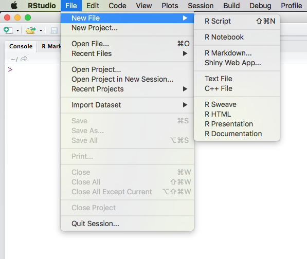
Choose R Markdown, give the document a title, and a text editor window will then open containing the R Markdown template:

(Click to enlarge.)

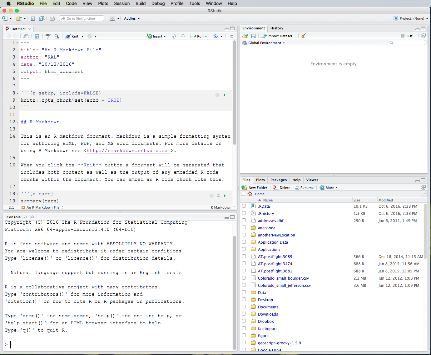
You should now have 4 panes open in RStudio. The content of the panes can be customized under Pane Layout in RStudio Preferences. What you see in the above screenshot is the default layout. The upper-left pane is a text editor containing the R Markdown document we just created. This editor can also be used to create R scripts and various other plain-text source files. Below the editor is a pane containing the R Console. This is exactly the same console that you would get if you ran R by itself, independently from RStudio. (The Console pane contains an instance of R running inside of RStudio. You can have multiple instances of RStudio running at once, each running its own separate instance of R.) You can enter R commands directly into the Console, and text output from R commands will also appear here. In the upper right pane are tabs for the Environment (containing variables and other data structures created during the session) and History (a list of all R commands entered during the session). In the lower-right pane are tabs for Files (your computer’s filesystem), Plots (graphics created by R), Packages (a tool for installing and updating R packages), Help (the R help system), and the Viewer (containing output from rendering R Markdown files and R Notebooks).

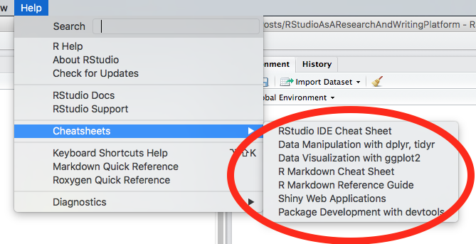
Of course, there is a very nice RStudio Cheat Sheet. The RStudio Help menu has links to additional very nice cheat sheets:

You can also access a Markdown Quick Reference from the RStudio Help menu. This will open up in the RStudio Help tab. You can copy-paste Markdown syntax from the Quick Reference into your R Markdown document. (Sadly, RStudio does not have Markdown syntax built into its editor, at least at the time of this writing.)

The first part of the as-yet-unnamed R Markdown file looks like this:

---
title: "An R Markdown File"
author: "RAL"
date: "10/14/2016"
output: html_document
---

This is called the YAML header. YAML (YAML Ain’t Markup Language) is a human friendly data serialization standard for all programming languages. In R Markdown, the YAML header (which is optional) is placed at the top of the document between lines that start with three dashes (---) and contains metadata for the document (e.g., title, author, date) and other options that control how the document is rendered.

Besides the YAML header, R Markdown documents contain either text or code chunks. Text is formatted using R Markdown syntax. R code chunks are made with three backticks immediately followed on the same line by an r in braces. End the chunk with three more backticks, on a separate line:

```{r}
paste("Hello", "World!")

``` 

The backtick symbol is located to the left of the numeral 1 on your keyboard. It is NOT a single apostrophe (').

Additional R options can be placed inside of the braces, for example:

```{r, echo=FALSE}
summary(cars)
```

The R option echo=FALSE will display the output of a code chunk but not the underlying R code.

All of the R code for a chunk must be inside of the space defined by the two lines of backticks.

At the top of the editor window is a toolbar:

Drop down the menu next to the Knit icon, and you will see options for rendering the R Markdown document into publication-quality output:

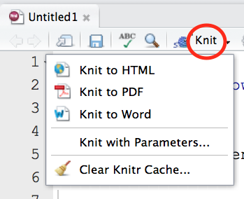
This function is called Knit because it invokes an R package called knitr that “knits” the Markdown-formatted text, relevant YAML content, and R code chunks together into a rendered document.

Try knitting the document into HTML, PDF, and Word formats. You will first need to give the R Markdown file a name, if you haven’t already done so. The default R Markdown file name extension is Rmd. The HTML rendering will appear in the RStudio Viewer pane. If it appears in a separate window, drop down the gear icon next to the knit button and select Preview in Viewer Pane. PDF output will open in a separate PDF viewer window. When you render the document to Microsoft Word format, it will open up in Microsoft Word. HTML, PDF, and Word files having the same name as your R Markdown document will be saved in your working directory.

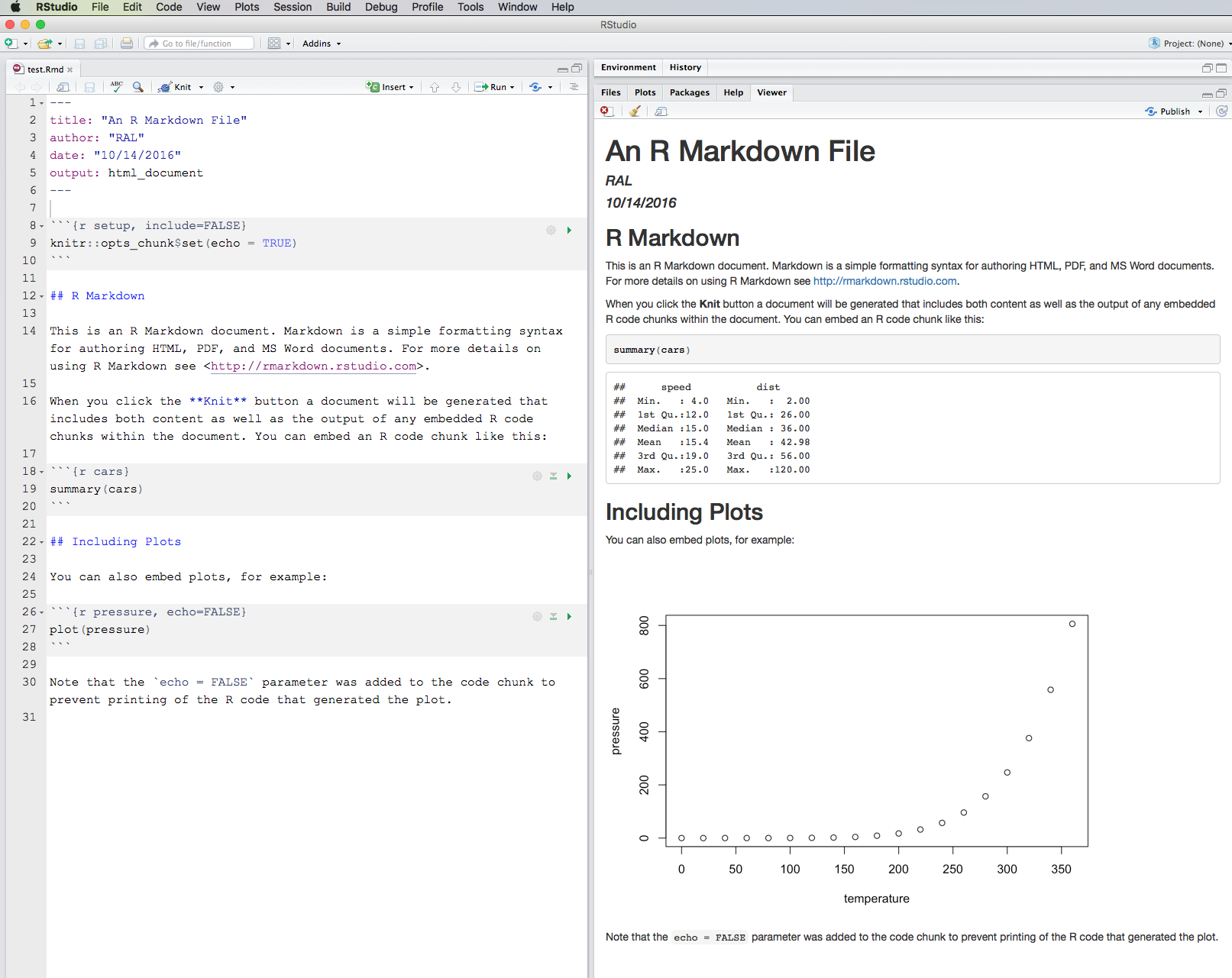
Let’s look at an HTML rendering:

(Click to enlarge).

In the above screenshot I have maximized the Editor and Viewer panes so we can see them side-by-side. The title, author, and date contained in the YAML header appear in the rendered document, but the YAML statement output: html_document does not because it is a formatting command, not printable text. Regular text appears in the HTML as formatted by R Markdown syntax. Text and graphical output produced by R code chunks appears in the rendered document at the point where the code chunks were placed in the original R Markdown document. Display of the code itself can be turned off in the rendered document by use of the echo=FALSE parameter in the code chunk:

```{r pressure, echo=FALSE}
plot(pressure)
```

If you knit the R Markdown document to HTML, PDF, and Word formats, you will notice that the YAML header in the R Markdown document has been modified:

---
title: "An R Markdown File"
author: "RAL"
date: "10/14/2016"
output:
  word_document: default
  pdf_document: default
  html_document: default
---

RStudio inserts additional formatting parameters into the YAML header to control how the document is rendered. You can do this manually as well, simply by editing the YAML header directly, in the editor. For example, to control the size of R graphics in Microsoft Word, add this to the YAML header:

output:
  word_document:
    fig_width: 3
    fig_height: 3

This will cause figures in the resulting Word file to be sized at 3 by 3 inches. You can also set YAML options interactively, by clicking the gear icon to the right of the Knit button, and choosing Output Options:

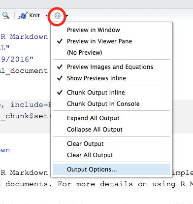
This will give you a dialog box from which you can choose the various output formats and set things like figure size, inclusion of figure captions, etc.:

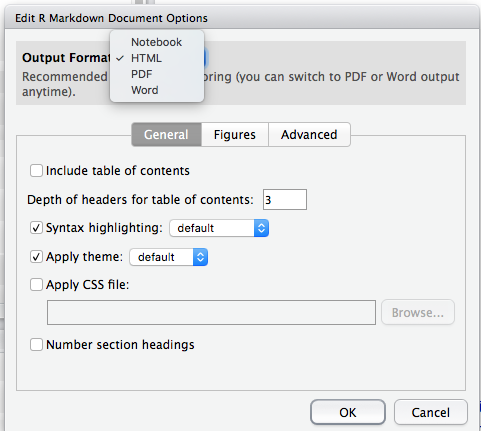
When you make selections from the Output Options dialog, RStudio will make the appropriate changes to the YAML header in the R Markdown document. You can also edit those parameters directly in the YAML header, as mentioned earlier.

See RStudio Formats for more formats and YAML options for rendering R Markdown documents.